目录
- Probability and Bayes’ Rule
- Introduction
- Probabilities
- Probability of the intersection
- Bayes’ Rule
- Conditional Probabilities
- Bayes’ Rule
- Quiz: Bayes’ Rule Applied
- Naïve Bayes Introduction
- Naïve Bayes for Sentiment Analysis
- P ( w i ∣ c l a s s ) P(w_i|class) P(wi∣class)
- Naïve Bayes
- Laplacian Smoothing
- Laplacian Smoothing
- Introducing P ( w i ∣ c l a s s ) P(w_i|class) P(wi∣class) with smoothing
- Log Likelihood
- Ratio of probabilities
- Naïve Bayes’ inference
- Log Likelihood, Part1
- Calculating Lambda
- Summary
- Log Likelihood, Part 2
- Training Naïve Bayes
- Testing Naïve Bayes
- Predict using Naïve Bayes
- Testing Naïve Bayes
- Applications of Naïve Bayes
- Naïve Bayes Assumptions
- Error Analysis
- Punctuation
- Removing Words
- Adversarial attacks
Probability and Bayes’ Rule
概率与条件概率及其数学表达
贝叶斯规则(应用于不同领域,包括 NLP)
建立自己的 Naive-Bayes 推文分类器
Introduction
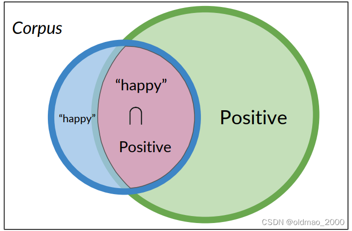
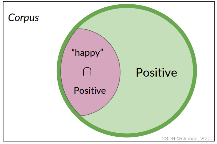
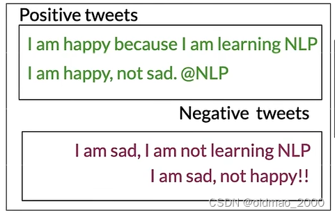
假设我们有一个推文语料库,里面包含正面和负面情感的推文:
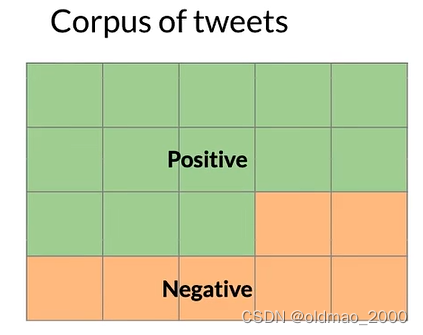
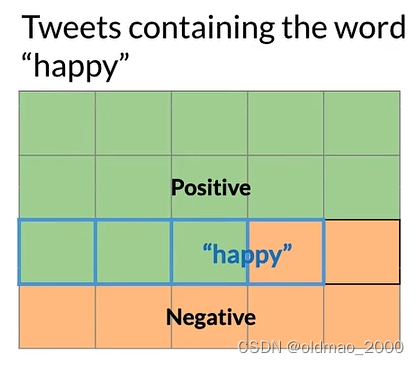
某个单词例如:happy,可能出现在正面或负面情感的推文中:
下面我们用数学公式来表示上面的概率描述。
Probabilities
A
A
A表示正面的推文,则正面的推文发生的概率可以表示为:
P
(
A
)
=
P
(
P
o
s
i
t
i
v
e
)
=
N
p
o
s
/
N
P(A)=P(Positive)=N_{pos}/N
P(A)=P(Positive)=Npos/N
以上图为例:
P
(
A
)
=
N
p
o
s
/
N
=
13
/
20
=
0.65
P(A)=N_{pos}/N=13/20=0.65
P(A)=Npos/N=13/20=0.65
而负面推文发生的概率可以表示为:
P
(
N
e
g
a
t
i
v
e
)
=
1
−
P
(
P
o
s
i
t
i
v
e
)
=
0..35
P(Negative)=1-P(Positive)=0..35
P(Negative)=1−P(Positive)=0..35
happy可能出现在正面或负面情感的推文中可以表示为
B
B
B:
则
B
B
B发生概率可以表示为:
P
(
B
)
=
P
(
h
a
p
p
y
)
=
N
h
a
p
p
y
/
N
P
(
B
)
=
4
/
20
=
0.2
P(B) = P(happy) = N_{happy}/N\\ P(B) =4/20=0.2
P(B)=P(happy)=Nhappy/NP(B)=4/20=0.2
Probability of the intersection
下面表示正面推文且包含单词happy可图形化表示为:
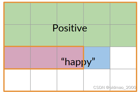
也可以用交集的形式表示:
P
(
A
∩
B
)
=
P
(
A
,
B
)
=
3
20
=
0.15
P(A\cap B)=P(A,B)=\cfrac{3}{20}=0.15
P(A∩B)=P(A,B)=203=0.15
语料库中有20条推文,其中有3条被标记为积极且同时包含单词happy
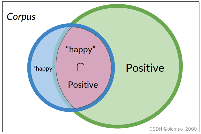
Bayes’ Rule
Conditional Probabilities
如果我们在三亚,并且现在是冬天,你可以猜测天气如何,那么你的猜测比只直接猜测天气要准确得多。
用推文的例子来说:
如果只考虑包含单词happy的推文(4条),而不是整个语料库,考虑这个里面包含正面推文的概率:
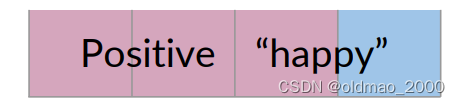
P
(
A
∣
B
)
=
P
(
P
o
s
i
t
i
v
e
∣
“
h
a
p
p
y
"
)
P
(
A
∣
B
)
=
3
/
4
=
0.75
P(A|B)=P(Positive|“happy")\\ P(A|B)=3/4=0.75
P(A∣B)=P(Positive∣“happy")P(A∣B)=3/4=0.75
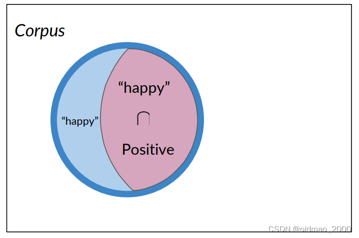
反过来说,只考虑正面推文,看其出现happy单词的推文概率:
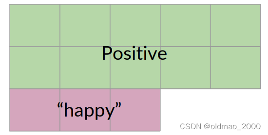
P
(
B
∣
A
)
=
P
(
“
h
a
p
p
y
”
∣
P
o
s
i
t
i
v
e
)
P
(
B
∣
A
)
=
3
/
13
=
0.231
P(B | A) = P(“happy”| Positive) \\ P(B | A) = 3 / 13 = 0.231
P(B∣A)=P(“happy”∣Positive)P(B∣A)=3/13=0.231
从上面例子可以看到:条件概率可以被解释为已知事件A已经发生的情况下,结果B发生的概率,或者从集合A中查看一个元素,它同时属于集合B的概率。
Probability of B, given A happened
Looking at the elements of set A, the chance that one also belongs to set B
P
(
P
o
s
i
t
i
v
e
∣
“
h
a
p
p
y
"
)
=
P
(
P
o
s
i
t
i
v
e
∩
“
h
a
p
p
y
"
)
P
(
“
h
a
p
p
y
"
)
P(Positive|“happy")=\cfrac{P(Positive\cap “happy")}{P(“happy")}
P(Positive∣“happy")=P(“happy")P(Positive∩“happy")
Bayes’ Rule
使用条件概率推导贝叶斯定理
同理:
P
(
P
o
s
i
t
i
v
e
∣
“
h
a
p
p
y
"
)
=
P
(
P
o
s
i
t
i
v
e
∩
“
h
a
p
p
y
"
)
P
(
“
h
a
p
p
y
"
)
P(Positive|“happy")=\cfrac{P(Positive\cap “happy")}{P(“happy")}
P(Positive∣“happy")=P(“happy")P(Positive∩“happy")
P
(
“
h
a
p
p
y
"
∣
P
o
s
i
t
i
v
e
)
=
P
(
“
h
a
p
p
y
"
∩
P
o
s
i
t
i
v
e
)
P
(
P
o
s
i
t
i
v
e
)
P(“happy"|Positive)=\cfrac{P( “happy"\cap Positive)}{P(Positive)}
P(“happy"∣Positive)=P(Positive)P(“happy"∩Positive)
上面两个式子的分子表示的数量是一样的。
有了以上公式则可以推导贝叶斯定理。
P
(
P
o
s
i
t
i
v
e
∣
“
h
a
p
p
y
"
)
=
P
(
“
h
a
p
p
y
"
∣
P
o
s
i
t
i
v
e
)
×
P
(
P
o
s
i
t
i
v
e
)
P
(
“
h
a
p
p
y
"
)
P(Positive|“happy")=P(“happy"|Positive)\times\cfrac{P(Positive)}{P(“happy")}
P(Positive∣“happy")=P(“happy"∣Positive)×P(“happy")P(Positive)
通用形式为:
P
(
X
∣
Y
)
=
P
(
Y
∣
X
)
×
P
(
X
)
P
(
Y
)
P(X|Y)=P(Y|X)\times \cfrac{P(X)}{P(Y)}
P(X∣Y)=P(Y∣X)×P(Y)P(X)
Quiz: Bayes’ Rule Applied
Suppose that in your dataset, 25% of the positive tweets contain the word ‘happy’. You also know that a total of 13% of the tweets in your dataset contain the word ‘happy’, and that 40% of the total number of tweets are positive. You observe the tweet: '‘happy to learn NLP’. What is the probability that this tweet is positive?
A: P(Positive | “happy” ) = 0.77
B: P(Positive | “happy” ) = 0.08
C: P(Positive | “happy” ) = 0.10
D: P(Positive | “happy” ) = 1.92
答案:A
Naïve Bayes Introduction
学会使用Naïve Bayes来进行二分类(使用概率表)
Naïve Bayes for Sentiment Analysis
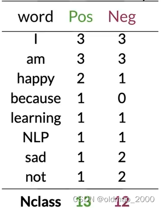
假设有以下语料:
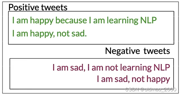
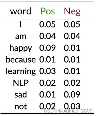
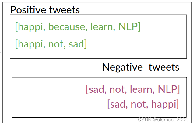
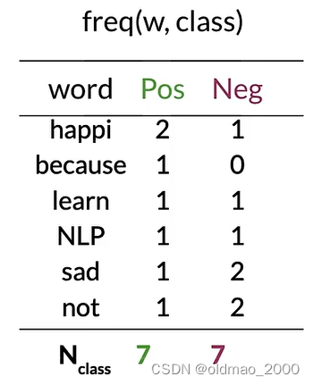
按C1W1中提到方法提取词库,并统计正负面词频:
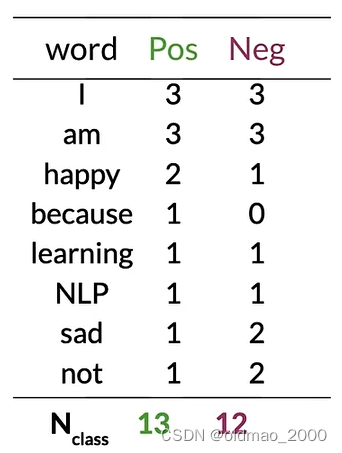
P ( w i ∣ c l a s s ) P(w_i|class) P(wi∣class)
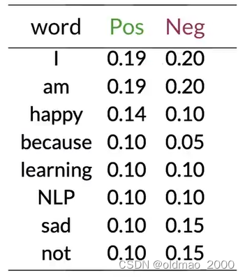
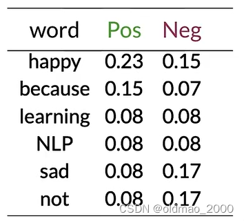
将类别中每个单词的频率除以它对应的类别中单词的总数。
例如:对于单词"I",正面类别的条件概率将是3/13:
p
(
I
∣
P
o
s
)
=
3
13
=
0.24
p(I|Pos)=\cfrac{3}{13}=0.24
p(I∣Pos)=133=0.24
对于负面类别中的单词"I",可以得到3/12:
p
(
I
∣
N
e
g
)
=
3
12
=
0.25
p(I|Neg)=\cfrac{3}{12}=0.25
p(I∣Neg)=123=0.25
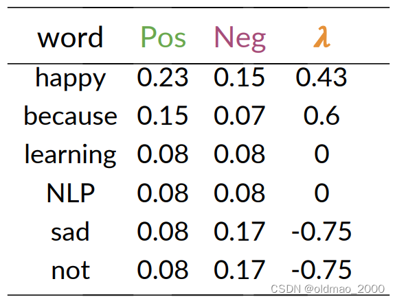
将以上内容保存为表(because的Neg概率不太对,应该是0):
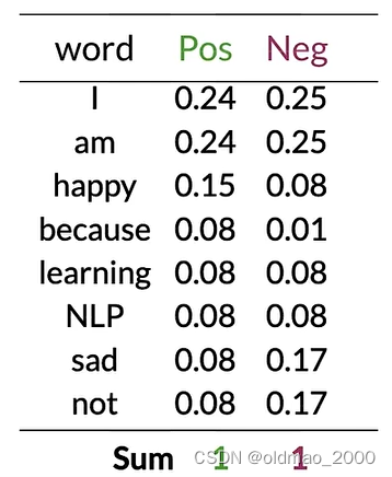
可以看到有很多单词(中性词)在表中的Pos和Neg的值大约相等(Pos≈Neg),例如:I、am、learning、NLP。
这些具有相等概率的单词对情感没有任何贡献。
而单词happy、sad、not的Pos和Neg的值差异很大,这些词对于确定推文的情感具有很大影响,绿色是积极影响,紫色是负面影响。
对于单词because,其
p
(
I
∣
N
e
g
)
=
0
12
=
0
p(I|Neg)=\cfrac{0}{12}=0
p(I∣Neg)=120=0
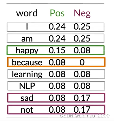
这情况在计算贝叶斯概率的时候会出现分母为0的情况,为避免这个情况发生,可以引入平滑处理。
Naïve Bayes
假如有以下推文:
I am happy today; I am learning.
按上面的计算方式得到词表以及其Pos和Neg的概率值:
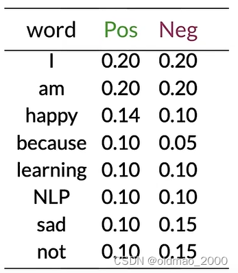
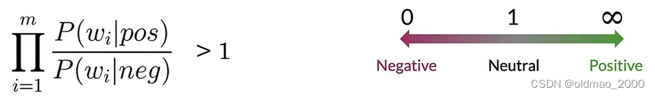
使用以下公式计算示例推文的情感:
∏
i
=
1
m
P
(
w
i
∣
p
o
s
)
P
(
w
i
∣
n
e
g
)
\prod_{i=1}^m\cfrac{P(w_i|pos)}{P(w_i|neg)}
i=1∏mP(wi∣neg)P(wi∣pos)
就是计算推文每个单词的第二列比上第三列,然后连乘。
示例推文today不在词表中,忽略,其他单词带入公式:
0.20
0.20
×
0.20
0.20
×
0.14
0.10
×
0.20
0.20
×
0.20
0.20
×
0.10
0.10
=
0.14
0.10
=
1.4
>
1
\cfrac{0.20}{0.20}\times\cfrac{0.20}{0.20}\times\cfrac{0.14}{0.10}\times\cfrac{0.20}{0.20}\times\cfrac{0.20}{0.20}\times\cfrac{0.10}{0.10}=\cfrac{0.14}{0.10}=1.4>1
0.200.20×0.200.20×0.100.14×0.200.20×0.200.20×0.100.10=0.100.14=1.4>1
可以看到,中性词对预测结果没有任何作用,最后结果大于1,表示示例推文是正面的。
Laplacian Smoothing
Laplacian Smoothing主要用于以下目的:
避免零概率问题:在统计语言模型中,某些词或词序列可能从未在训练数据中出现过,导致其概率为零。拉普拉斯平滑通过为所有可能的事件分配一个非零概率来解决这个问题。
概率分布估计:拉普拉斯平滑提供了一种简单有效的方法来估计概率分布,即使在数据不完整或有限的情况下。
平滑处理:它通过为所有可能的事件添加一个小的常数(通常是1),来平滑概率分布,从而减少极端概率值的影响。
提高模型的泛化能力:通过避免概率为零的情况,拉普拉斯平滑有助于提高模型对未见数据的泛化能力。
简化计算:拉普拉斯平滑提供了一种简单的方式来调整概率,使得计算和实现相对容易。
Laplacian Smoothing
计算给定类别下一个词的条件概率的表达式是词在语料库中出现的频率:
P
(
w
i
∣
c
l
a
s
s
)
=
f
r
e
q
(
w
i
,
c
l
a
s
s
)
N
c
l
a
s
s
c
l
a
s
s
∈
{
P
o
s
i
t
i
v
e
,
N
e
g
a
t
i
v
e
}
P(w_i|class)=\cfrac{freq(w_i,class)}{N_{class}}\quad class\in\{Positive,Negative\}
P(wi∣class)=Nclassfreq(wi,class)class∈{Positive,Negative}
其中
N
c
l
a
s
s
N_{class}
Nclass是frequency of all words in class
加入平滑项后公式写为:
P
(
w
i
∣
c
l
a
s
s
)
=
f
r
e
q
(
w
i
,
c
l
a
s
s
)
+
1
N
c
l
a
s
s
+
V
c
l
a
s
s
P(w_i|class)=\cfrac{freq(w_i,class)+1}{N_{class}+V_{class}}
P(wi∣class)=Nclass+Vclassfreq(wi,class)+1
V
c
l
a
s
s
V_{class}
Vclass是number of unique words in class
分子项+1避免了概率为0的情况,但是会导致总概率不等于1的情况,为了避免这个情况,在分母中加了
V
c
l
a
s
s
V_{class}
Vclass
Introducing P ( w i ∣ c l a s s ) P(w_i|class) P(wi∣class) with smoothing
使用之前的例子。
上表中共有8个不同单词,
V
=
8
V=8
V=8
对于单词I则有:
P
(
I
∣
P
o
s
)
=
3
+
1
13
+
8
=
0.19
P
(
I
∣
N
e
g
)
=
3
+
1
12
+
8
=
0.20
P(I|Pos)=\cfrac{3+1}{13+8}=0.19\\ P(I|Neg)=\cfrac{3+1}{12+8}=0.20
P(I∣Pos)=13+83+1=0.19P(I∣Neg)=12+83+1=0.20
同理可以计算出其他单词平滑厚度结果:
虽然结果已经四舍五入,但是两列概率值总和还是为1
Log Likelihood
Ratio of probabilities
根据之前讲的内容,我们知道每个单词可以按其Pos和Neg的值的差异分为三类,正面、负面和中性词。
我们把这个差异用下面公式表示:
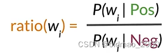
然后,我们可以计算上面概率表中的ratio(吐槽一下,这里because的概率不知道怎么搞的老是变来变去)
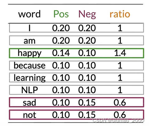
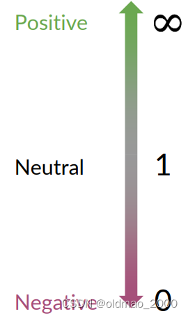
ratio取值与分类的关系很简单:
Naïve Bayes’ inference
下面给出完整的朴素贝叶斯二元分类公式:
P
(
p
o
s
)
P
(
n
e
g
)
∏
i
=
1
m
P
(
w
i
∣
p
o
s
)
P
(
w
i
∣
n
e
g
)
>
1
c
l
a
s
s
∈
{
p
o
s
,
n
e
g
}
w
→
Set of m words in a tweet
\cfrac{P(pos)}{P(neg)}\prod_{i=1}^m\cfrac{P(w_i|pos)}{P(w_i|neg)}>1\quad class\in\{pos,neg\}\quad w\rightarrow\text{Set of m words in a tweet}
P(neg)P(pos)i=1∏mP(wi∣neg)P(wi∣pos)>1class∈{pos,neg}w→Set of m words in a tweet
左边一项其实是先验概率,如果数据集中正负样本差不多,则该项比值为1,可以忽略。这个比率可以看作是模型在没有任何其他信息的情况下,倾向于认为推文是正面或负面情感的初始信念。;
右边一项之前已经推导过。这是条件概率的乘积。对于推文中的每个词
w
i
,
i
=
1
,
2
,
⋯
,
m
w_i,i=1,2,\cdots,m
wi,i=1,2,⋯,m(m 是推文中的词的数量),这个乘积计算了在正面情感条件下该词出现的概率与在负面情感条件下该词出现的概率的比值。这个乘积考虑了推文中所有词的证据
如果这个乘积大于1,那么模型认为推文更可能是正面情感;如果小于1,则更可能是负面情感。
Log Likelihood, Part1
上面的朴素贝叶斯二元分类公式使用了连乘的形式,对于计算上说,小数的连乘会使得计算出现underflow,根据对数性质:
log
(
a
∗
b
)
=
log
(
a
)
+
log
(
b
)
\log(a*b)=\log(a)+\log(b)
log(a∗b)=log(a)+log(b)
可以将连乘转化成为连加的形式,同样对公式求对数得到:
log
(
P
(
p
o
s
)
P
(
n
e
g
)
∏
i
=
1
m
P
(
w
i
∣
p
o
s
)
P
(
w
i
∣
n
e
g
)
)
=
log
P
(
p
o
s
)
P
(
n
e
g
)
+
∑
i
=
1
m
log
P
(
w
i
∣
p
o
s
)
P
(
w
i
∣
n
e
g
)
\log\left(\cfrac{P(pos)}{P(neg)}\prod_{i=1}^m\cfrac{P(w_i|pos)}{P(w_i|neg)}\right)=\log\cfrac{P(pos)}{P(neg)}+\sum_{i=1}^m\log\cfrac{P(w_i|pos)}{P(w_i|neg)}
log(P(neg)P(pos)i=1∏mP(wi∣neg)P(wi∣pos))=logP(neg)P(pos)+i=1∑mlogP(wi∣neg)P(wi∣pos)
也就是:log prior + log likelihood
我们将第一项成为:
λ
\lambda
λ
Calculating Lambda
根据上面的内容计算实例推文的lambda:
tweet: I am happy because I am learning.
先计算出概率表:
然后根据公式计算出每个单词的
λ
\lambda
λ:
λ
(
w
)
=
log
P
(
w
∣
p
o
s
)
P
(
w
∣
n
e
g
)
\lambda(w)=\log\cfrac{P(w|pos)}{P(w|neg)}
λ(w)=logP(w∣neg)P(w∣pos)
例如对于第一个单词:
λ
(
I
)
=
log
0.05
0.05
=
log
(
1
)
=
0
\lambda(I)=\log\cfrac{0.05}{0.05}=\log(1)=0
λ(I)=log0.050.05=log(1)=0
happy:
λ
(
h
a
p
p
y
)
=
log
0.09
0.01
=
log
(
9
)
=
2.2
\lambda(happy)=\log\cfrac{0.09}{0.01}=\log(9)=2.2
λ(happy)=log0.010.09=log(9)=2.2
以此类推:
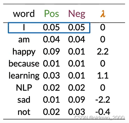
可以看到,这里我们也可以根据
λ
\lambda
λ值来判断正负面和中性词。
Summary
对于正负面、中性词,这里给出两种判断方式(Word sentiment):
r
a
t
i
o
(
w
)
=
P
(
w
∣
p
o
s
)
P
(
w
∣
n
e
g
)
ratio(w)=\cfrac{P(w|pos)}{P(w|neg)}
ratio(w)=P(w∣neg)P(w∣pos)
λ
(
w
)
=
log
P
(
w
∣
p
o
s
)
P
(
w
∣
n
e
g
)
\lambda(w)=\log\cfrac{P(w|pos)}{P(w|neg)}
λ(w)=logP(w∣neg)P(w∣pos)
这里要明白,为什么要使用第二种判断方式:避免underflow(下溢)
Log Likelihood, Part 2
有了
λ
\lambda
λ值,接下来可以计算对数似然,对于以下推文:
I am happy because I am learning.
其每个单词
λ
\lambda
λ值在上面的图中,整个推文的对数似然值就是做累加:
0
+
0
+
2.2
+
0
+
0
+
0
+
1.1
=
3.3
0+0+2.2+0+0+0+1.1=3.3
0+0+2.2+0+0+0+1.1=3.3
从前面我们可以知道,概率比值以及对数似然的值如何区分正负样本:
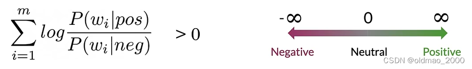
这里的推文对数似然的值为3.3,是一个正面样本。
Training Naïve Bayes
这里不用GD,只需简单五步完成训练模型。
Step 0: Collect and annotate corpus
Step 1: Preprocess
包括:
Lowercase
Remove punctuation, urls, names
Remove stop words
Stemming
Tokenize sentences
Step 2: Word count
Step 3:
P
(
w
∣
c
l
a
s
s
)
P(w|class)
P(w∣class)
这里
V
c
l
a
s
s
=
6
V_{class}=6
Vclass=6
根据公式:
f
r
e
q
(
w
,
c
l
a
s
s
)
+
1
N
c
l
a
s
s
+
V
c
l
a
s
s
\cfrac{freq(w,class)+1}{N_{class}+V_{class}}
Nclass+Vclassfreq(w,class)+1
计算概率表:
Step 4: Get lambda
根据公式:
λ
(
w
)
=
log
P
(
w
∣
p
o
s
)
P
(
w
∣
n
e
g
)
\lambda(w)=\log\cfrac{P(w|pos)}{P(w|neg)}
λ(w)=logP(w∣neg)P(w∣pos)
得到:
Step 5: Get the log prior
估计先验概率,分别计算:
D
p
o
s
D_{pos}
Dpos = Number of positive tweets
D
n
e
g
D_{neg}
Dneg = Number of negative tweets
log prior
=
log
D
p
o
s
D
n
e
g
\text{log prior}=\log\cfrac{D_{pos}}{D_{neg}}
log prior=logDnegDpos
注意:
If dataset is balanced,
D
p
o
s
=
D
n
e
g
D_{pos}=D_{neg}
Dpos=Dneg and
log prior
=
0
\text{log prior}=0
log prior=0.
对应正负样本不均衡的数据库,先验概率不能忽略
总的来看是六步:
- Get or annotate a dataset with positive and negative tweets
- Preprocess the tweets: p r o c e s s _ t w e e t ( t w e e t ) ➞ [ w 1 , w 2 , w 3 , . . . ] process\_tweet(tweet) ➞ [w_1 , w_2 , w_3 , ...] process_tweet(tweet)➞[w1,w2,w3,...]
- Compute freq(w, class),注意要引入拉普拉斯平滑
- Get P(w | pos), P(w | neg)
- Get λ(w)
- Compute log prior = log(P(pos) / P(neg))
Testing Naïve Bayes
Predict using Naïve Bayes
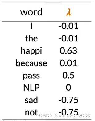
进行之前的步骤,我们完成了词典中每个单词对数似然λ(w)的计算,并形成了字典。
假设我们数据集中正负样本基本均衡,可以忽略对数先验概率(
log prior
=
0
\text{log prior}=0
log prior=0)
对于推文:
[I, pass, the , NLP, interview]
计算其对数似然为:
s
c
o
r
e
=
−
0.01
+
0.5
−
0.01
+
0
+
log prior
=
0.48
score = -0.01+0.5-0.01+0+\text{log prior}=0.48
score=−0.01+0.5−0.01+0+log prior=0.48
其中interview为未知词,忽略。
也就是是预测值为0.48>0,该推文是正面的。
Testing Naïve Bayes
假设有验证集数据:
X
v
a
l
X_{val}
Xval和标签
Y
v
a
l
Y_{val}
Yval
计算
λ
\lambda
λ和log prior,对于未知词要忽略(也就相当于看做是中性词)
计算
s
c
o
r
e
=
p
r
e
d
i
c
t
(
X
v
a
l
,
λ
,
log prior
)
score=predict(X_{val},\lambda,\text{log prior})
score=predict(Xval,λ,log prior)
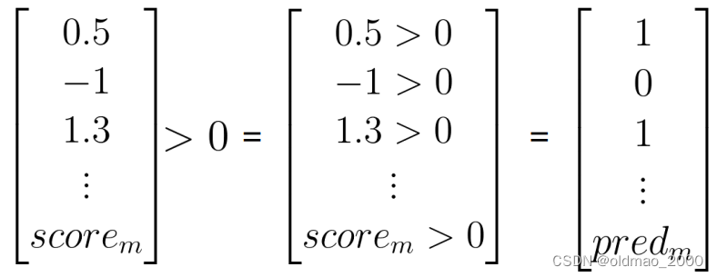
判断推文情感:
p
r
e
d
=
s
c
o
r
e
>
0
pred = score>0
pred=score>0
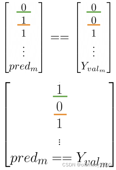
计算模型正确率:
1
m
∑
i
=
1
m
(
p
r
e
d
i
=
=
Y
v
a
l
i
)
\cfrac{1}{m}\sum_{i=1}^m(pred_i==Y_{val_i})
m1i=1∑m(predi==Yvali)
Applications of Naïve Bayes
除了Sentiment analysis
Naïve Bayes常见应用还包括:
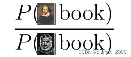
● Author identification
如果有两个大型文集,分别由不同的作者撰写,可以训练一个模型来识别新文档是由哪一位写的。
例如:你手头上有一些莎士比亚的作品和海明威的作品,你可以计算每个词的Lambda值,以预测个新词被莎士比亚使用的可能性,或者被海明威使用的可能性。
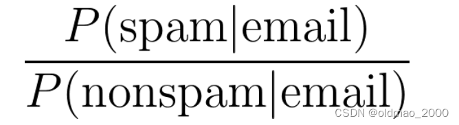
●Spam filtering:
● Information retrieval
朴素贝叶斯最早的应用之一是在数据库中根据查询中的关键字将文档筛选为相关和不相关的文档。
这里只需要计算文档的对数似然,因为先验是未知的。
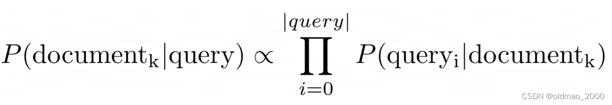
然后根据阈值判断是否查询文档:

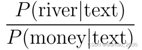
● Word disambiguation
假设单词在文中有两种含义,词义消岐可以判断单词在上下文的含义。

bank有河岸和银行两种意思。
Naïve Bayes Assumptions
朴素贝叶斯是一个非常简单的模型,它不需要设置任何自定义参数,因为它对数据做了一些假设。
● Independence
● Relative frequency in corpus
对于独立性,朴素贝叶斯假设文本中的词语是彼此独立的。看下面例子:
“It is sunny and hot in the Sahara desert.”
单词sunny 和hot 是有关联性的,两个词语在一起可能与其所描述的事物有关,例如:海滩、甜点等。
朴素贝叶斯独立性的假设可能会导致对个别词语的条件概率估计不准确。
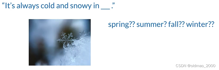
例如上图中,winter的概率明显要高于其他单词,但朴素贝叶斯则认为四个单词概率一样。
另外一个问题是依赖于训练数据集的分布。
理想的数据集中应该包含与随机样本相同比例的积极和消极推文,但是实际的推文中,正面推文要比负面推文出现频率要更高。这样训练出来的模型会被戴上有色眼镜。
Error Analysis
造成预测失败的原因有三种:
● Removing punctuation and stop words
● Word order
● Adversarial attacks
Punctuation
Tweet: My beloved grandmother : (
经过标点处理后:processed_tweet: [belov, grandmoth]
我亲爱的祖母,本来是正面推文,但是后面代表悲伤的emoj被过滤掉了。如果换成感叹号那就不一样。
Removing Words
Tweet: This is not good, because your attitude is not even close to being nice.
去掉停用词后:processed_tweet: [good, attitude, close, nice]
Tweet: I am happy because I do not go.
Tweet: I am not happy because I did go.
上面一个是正面的(I am happy),后面一个是负面的(I am not happy)
否定词和词序会导致预测错误。
Adversarial attacks
主要是Sarcasm, Irony and Euphemisms(讽刺、反讽和委婉语),天才Sheldon都不能李姐!!!
Tweet: This is a ridiculously powerful movie. The plot was gripping and I cried right through until the ending!
processed_tweet: [ridicul, power, movi, plot, grip, cry, end]
原文表达是正面的: 这是一部震撼人心的电影。情节扣人心弦,我一直哭到结局!
但处理后的单词却是负面的。
![[Vue3 + TS + Vite] ref 在 Template 与 Script 下的使用](/images/no-images.jpg)